Predicting Trade: The Upgrade That Wasn’t (Part 2)

Seasonal decomposition was supposed to fix the moving average. It didn’t — and finding out why was more useful than being right.

trade
forecasting
anomaly-detection
time-series
evaluation
python
Author

Aaron Koenigsberg

Published

July 10, 2026

NoteA note on how this was made

Part of an ongoing series on IMF International Merchandise Trade Statistics (IMTS) data, built by directing an AI research assistant: I set the questions, the evaluation design, and the interpretation; Claude wrote and ran the code. The analysis is what emerged from that back-and-forth — including the parts where my hypothesis turned out to be wrong.

Where we left off

Part 1 built a deliberately bad one-step-ahead forecaster — a 12-month moving average of partner export shares — and used its residuals to flag anomalies. It ended with a promise: Part 2 would bring in seasonal-trend decomposition (STL) to fix the moving average’s three failure modes (trend lag, calendar blindness, slow break absorption), and add a proper evaluation framework to measure whether any of this actually detects real-world events.

This post keeps that promise, with a twist: the seasonal upgrade loses to the naive baseline on every country, and the evaluation framework — the less glamorous half of the promise — turns out to be the thing that matters. By the end we’ll know why the obvious upgrade fails on this data, which “improvement” is just relabeling, and what genuinely works for the case every point-anomaly rule missed.

Setup

Same data and universe as Part 1: monthly goods-export shares to each country’s top 6 bilateral partners, for Ukraine, Venezuela, Yemen, Mexico, and Denmark, January 2017 through December 2025.

Four detectors

We compare four ways of turning each share series into anomaly flags. All four share the same flagging rule — \(|e_t| > 2\sigma\) on their residuals — so any difference comes from the model, not the threshold.

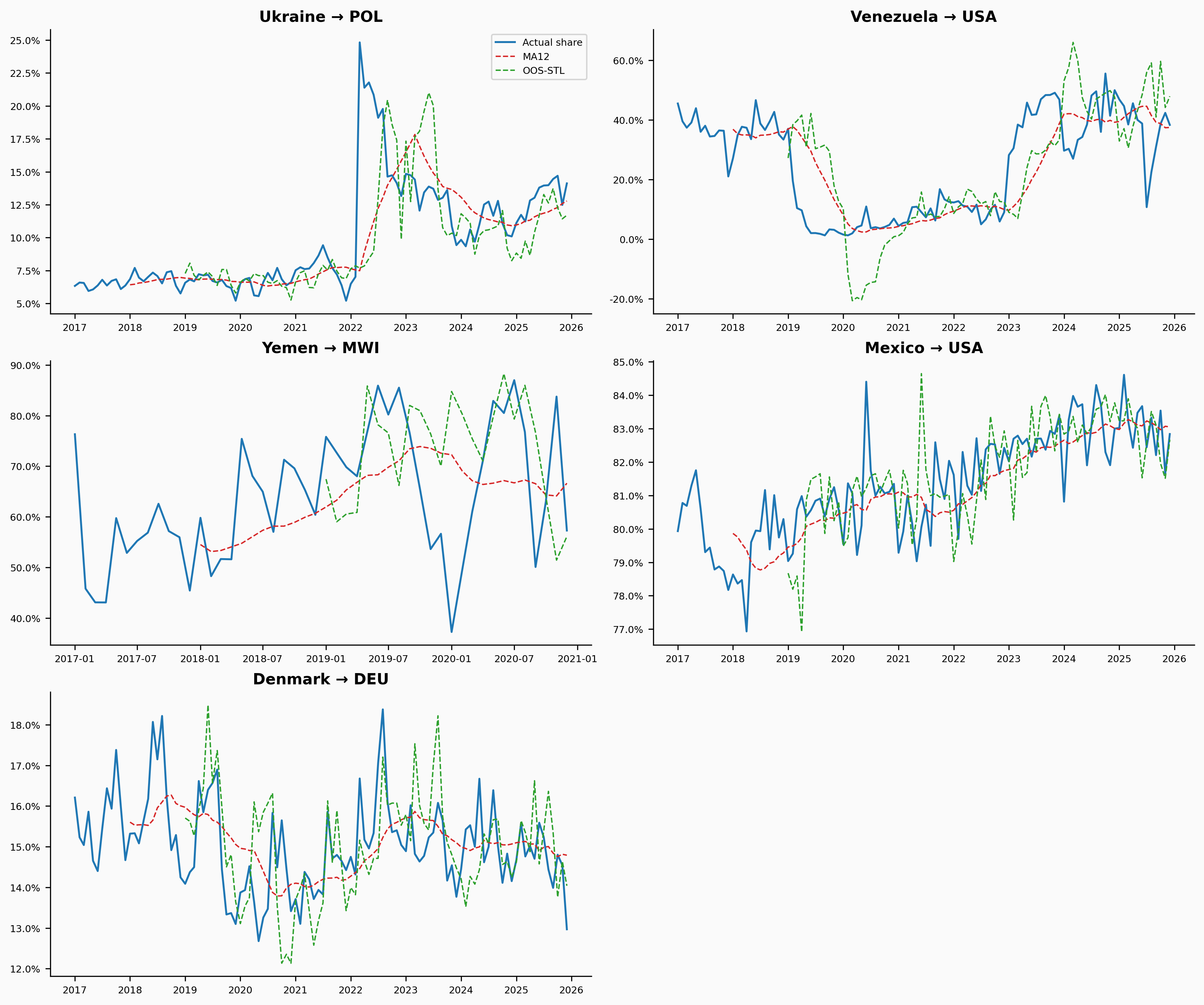
  1. MA12 (the Part 1 baseline). Prediction = trailing 12-month mean, shifted one period. Honest one-step-ahead: it only ever sees the past.

  2. Classic STL. Decompose the full series into trend + seasonal + remainder with STL, treat the remainder as the residual. This is the textbook approach — and it is not a forecast. The loess trend at month \(t\) is estimated using months after \(t\), so the remainder knows the future. It gets flattered by hindsight, and we include it precisely to measure how much.

  3. Out-of-sample STL (OOS-STL). At each month \(t\), fit STL only to data through \(t-1\), then forecast \(\hat{s}_t\) = last trend value + the seasonal component from the same calendar month a year earlier. An expanding-window, honest version of the decomposition idea.

  4. MA12 + seasonal. Deseasonalize with past-only STL, apply the trailing 12-month mean to the seasonally-adjusted series, re-add the seasonal. The hypothesis: keep the MA’s low-variance level estimate, fix only its calendar blindness.

Round 1: forecast accuracy

If the residuals are going to carry meaning, the forecasts need to be good. Here’s one-step-ahead MAE by country, averaged across each country’s partner series (classic STL is excluded — its “residuals” aren’t forecast errors).

Table 1: One-step-ahead mean absolute error in percentage points of export share. Bold = best.
Country MA12 (pp) OOS-STL (pp) MA12+seasonal (pp)
Ukraine 1.38 1.79 1.72
Venezuela 5.33 8.52 8.34
Yemen 8.05 12.16 12.06
Mexico 0.34 0.44 0.42
Denmark 0.71 0.95 0.93

The naive baseline wins everywhere — not by a little. OOS-STL is 25–60% worse; even the conservative MA12+seasonal hybrid loses on every country. Two seemingly obvious explanations fail quickly: it isn’t the warm-up window (both seasonal methods get the same one), and it isn’t robustness settings (robust STL is already being used).

Why: shares barely have seasons

Part 1 asserted that “trade patterns often have seasonal cycles” and counted calendar blindness as an MA failure mode. That’s true for trade levels. It is much less true for partner shares — seasonality hits the numerator and the denominator together, and mostly cancels in the ratio.

We can quantify that with the seasonal-strength measure from Hyndman & Athanasopoulos: \(F_s = \max\left(0,\ 1 - \frac{\mathrm{Var}(R_t)}{\mathrm{Var}(S_t + R_t)}\right)\), where \(S\) and \(R\) are the STL seasonal and remainder components. 0 means no seasonality; 1 means the seasonal component explains everything the trend doesn’t.

Table 2: Seasonal strength: total export levels vs. partner shares (median across each country’s top-6 partner series).
Country Levels (total exports) Shares (median, top-6 partners)
Ukraine 0.22 0.26
Venezuela 0.09 0.01
Yemen 0.46 0.04
Mexico 0.37 0.24
Denmark 0.57 0.22

Denmark’s total exports are strongly seasonal (0.57); its partner shares are not (0.22). Yemen’s shares have essentially zero seasonal structure. When the true seasonal signal is this weak, STL doesn’t extract signal — it manufactures it from noise, and the estimation variance it adds exceeds the variance it removes. The moving average never had a seasonality problem on this data representation. The lesson isn’t “STL is bad”; it’s that the upgrade was aimed at a failure mode this data doesn’t have.

Round 2: does anything detect real events?

Part 1 promised an evaluation framework, and this is where it earns its keep. For events with well-known dates, we check whether flags land inside the event window, and compare against the false-alarm rate everywhere else:

  • Ukraine: Russian invasion — February–May 2022
  • Venezuela: oil sanctions escalation — January–June 2019
  • Mexico & Denmark: COVID shock — March–June 2020
  • Yemen: no dated event (its disruption is chronic, not acute) — false alarms only

A 2σ rule flags ~4.6% of months by construction, so ~5% is the score a coin-flip detector gets. Hit rates need to clear that bar to mean anything.

Table 3: Event-window hit rate (flagged months inside window / eligible months) vs. false-alarm rate outside windows.
Country Method Hits Hit % False-alarm %
Ukraine MA12 9/22 41% 4.2%
Ukraine STL (classic) 13/22 59% 4.8%
Ukraine OOS-STL 9/22 41% 3.1%
Ukraine MA12+seasonal 10/22 45% 3.6%
Venezuela MA12 4/36 11% 5.7%
Venezuela STL (classic) 3/36 8% 7.7%
Venezuela OOS-STL 2/36 6% 6.0%
Venezuela MA12+seasonal 2/36 6% 6.0%
Yemen MA12 5.1%
Yemen STL (classic) 8.4%
Yemen OOS-STL 5.1%
Yemen MA12+seasonal 5.1%
Mexico MA12 6/24 25% 2.7%
Mexico STL (classic) 8/24 33% 4.2%
Mexico OOS-STL 4/24 17% 4.4%
Mexico MA12+seasonal 5/24 21% 3.8%
Denmark MA12 2/24 8% 4.2%
Denmark STL (classic) 3/24 12% 8.2%
Denmark OOS-STL 3/24 12% 4.8%
Denmark MA12+seasonal 6/24 25% 4.6%

Three things stand out:

Ukraine is detectable; Venezuela mostly isn’t. Every method beats the base rate handily on Ukraine (41–59% hit rates against a ~5% floor) — a violent overnight restructuring produces exactly the large one-month residuals that point rules catch. Venezuela’s 2019 collapse, which unfolded over months, stays near the base rate for every honest method. Same story as Part 1, now with numbers.

Classic STL’s edge is borrowed from the future. It posts the best Ukraine hit rate (59%) — and doubles Denmark’s false-alarm rate to 8.2%. The control country shouldn’t get more interesting under a better method. Hindsight decomposition sharpens real events and noise alike.

The honest seasonal methods buy nothing. OOS-STL and MA12+seasonal sit at or below MA12’s hit rates. Worse forecasts, no detection gain.

Figure 1: Ukraine, top-6 partner export shares. Markers above each panel: flagged months by method (red = MA12, purple = classic STL, green = OOS-STL, orange = MA12+seasonal). The 2022 invasion cluster is visible in every method; classic STL also sprinkles extra flags across quiet periods.
Figure 2: Denmark — the control. Under an honest method the flags are sparse and scattered; classic STL (purple) finds spurious structure.

Round 3: is a robust threshold the fix?

Part 1 flagged a masking problem: σ is estimated from residuals including the anomalies, so disrupted series get inflated thresholds. The standard fix is a robust scale estimate — median absolute deviation (MAD) instead of the standard deviation. Swapping it in raises hit rates everywhere… and raises false alarms nearly as fast. That should make you suspicious that we’ve improved anything.

The clean way to compare two threshold rules is at matched false-alarm rates: sweep the multiplier \(z\) for both rules and trace hit rate against false-alarm rate.

Figure 3: Hit rate vs. false-alarm rate as the threshold multiplier z sweeps 1.5–5.0, pooled across the four countries with dated events, MA12 residuals. The two rules trace nearly the same curve.

At any given false-alarm budget, the two rules deliver roughly the same hit rate. Switching to MAD at the same \(z\) isn’t a better detector — it’s a lower threshold wearing a robustness costume. If you want more hits, you could have just lowered \(z\). (MAD retains a real advantage the pooled curve understates: in heavily contaminated individual series it keeps single catastrophic months from swallowing the threshold. But as a headline fix, it’s relabeling.)

Round 4: the right tool for slow collapses

The Venezuela problem — sanctions bite, exports bleed away over 18 months, no single month looks extreme — is not a point-anomaly problem. It’s a sustained shift problem, and the classical tool for it is CUSUM (cumulative sum control charting): accumulate standardized residuals, subtracting a slack \(k\) each month, and alarm when the cumulative drift exceeds a decision interval \(h\). Small persistent errors that a 2σ rule ignores add up until CUSUM fires.

We run a standard two-sided CUSUM (\(k = 0.5\sigma\), \(h = 4\sigma\), robust σ, reset after each alarm) on the same MA12 residuals:

Figure 4: CUSUM on MA12 residuals for the two headline series. Top: export share. Bottom: CUSUM statistics with the ±4σ decision interval; red lines mark alarms.

The results on the headline cases are what the point rules couldn’t deliver:

  • Ukraine → Russia alarms in March 2022, one month after the invasion. It also alarms in mid-2020 and mid-2021 — not noise, but the tail of the long post-2014 decoupling grinding Russia’s share lower, which is exactly the kind of sustained drift CUSUM is built to accumulate.
  • Venezuela → USA alarms in March 2019, two months into the sanctions window that every 2σ rule scored near the base rate. Venezuela → India and → China alarm within the following two months, which is the rerouting story: barrels that stopped flowing to Houston went to Jamnagar instead.

The honest caveat: at these settings, an in-control Gaussian series should alarm roughly once every 14 years; our Denmark series alarm every 2–3 years. Trade-share residuals have heavier tails than the theory assumes (and the MA’s trend-lag feeds slow drifts into the accumulator), so the decision interval needs empirical calibration — the false-alarm arithmetic from Round 2 applies here too. CUSUM isn’t magic; it’s the right shape of detector for the right shape of disruption.

Scoreboard

Approach One-step accuracy Event detection Verdict
MA12 (naive baseline) Best Good on abrupt events Still the champion, annoyingly
Classic STL not a forecast Best-looking, borrowed from the future Use for description, never for detection claims
OOS-STL / MA12+seasonal 25–60% worse No gain Fixed a failure mode the data doesn’t have
MAD threshold n/a Same ROC curve as sd Relabeled threshold, not a better detector
CUSUM on MA12 residuals n/a Catches slow collapses point rules miss The real upgrade — calibrate before trusting

The methodological throughline: every “improvement” was evaluated against the boring baseline on out-of-sample accuracy and dated real-world events, and most of them failed. That’s not a disappointing result. The alternative — publishing the classic-STL flags because they looked sharpest — would have been a nicer-looking post describing a worse system, and nobody would have known until it was load-bearing.

What’s next

Three directions, in order of expected value:

  1. Model levels, not just shares. The seasonal signal that shares cancel out is alive in levels (strength 0.4–0.6). A level model with real seasonality, cross-checked against share-based flags, would separate “trade fell” from “trade reshuffled.”
  2. Calibrate CUSUM empirically. Set \(h\) per series from a false-alarm budget (via block bootstrap on pre-event residuals) rather than Gaussian theory, then re-score the event windows.
  3. Formal changepoint methods — PELT for retrospective segmentation, BOCPD for online detection — as the principled version of what CUSUM approximates, with the same honest evaluation harness ready to score them.

Data: IMF International Merchandise Trade Statistics, bulk flat file download. Events: Russian invasion of Ukraine (2022-02-24), US oil sanctions on Venezuela (2019-01-28), WHO COVID-19 pandemic declaration (2020-03-11).