Libraries

library(tidyverse)
library(ggridges)
library(ggiraph)
## Used by not read in:
# tibble

Transformations

To prep the data for analysis, I’m turning the year published into a date, rather than a character variable. Boardgamegeek has games published as far back as… hm… “0000-01-01”, so I’m going to be focusing on the period between 1950 and today.

games <- readRDS("~/Desktop/boardgamegeek/gamesDf.RDS")

gamesDf <- games %>%
  mutate(
    yearpublished = as.Date(paste(yearpublished, '01', '01', sep = '-'))
  ) %>%
  filter(
    yearpublished > '1950-01-01',
    yearpublished < '2018-01-01'
  )

Mechanics Over Time

I’ll start by using dplyr to summarize the data by yearpublished and boardgamemechanic. Then, I’m calculating the percent of total games per year in each mechanic.

mechanicDensities <-  gamesDf %>%
  filter(!is.na(boardgamemechanic)) %>%
  group_by(yearpublished, boardgamemechanic) %>%
  summarise(
    count = n()
  ) %>%
  mutate(
    percent = count/sum(count)
  ) 

To make the plot easier to read, I’m changing the default ordering of boardgamemechanic from the default (alphabetical) to be by overall count. Then I made a couple more swaps by hand.

mechanicOrder <-
  gamesDf %>%
  filter(!is.na(boardgamemechanic)) %>%
  group_by(boardgamemechanic) %>%
  summarize(count = n()) %>%
  arrange(count) %>%
  pull(boardgamemechanic)

mechanicOrder[c(51,50)] <- mechanicOrder[c(50,51)]
mechanicOrder[c(47,49)] <- mechanicOrder[c(49,47)]

mechanicDensities$boardgamemechanic <- factor(mechanicDensities$boardgamemechanic, 
                                              levels = mechanicOrder)

Finally, I’m using the ggridge package to draw a ridge plot. I found that to be the easiest and best way to show this many time series in a way that was easy to interpret.

ggplot(data = mechanicDensities, aes(x = yearpublished, y = boardgamemechanic, 
                                     group = boardgamemechanic, height = percent)) +
  geom_ridgeline(stat = 'identity', scale = 5) +
  theme_minimal()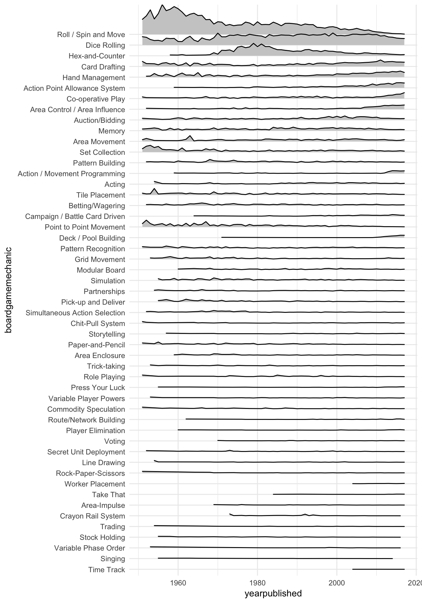

Observations

A few big things jump out immediately:

• Roll and move mechanics were pretty much the only mechanic for a long time, but are not common now.
• Dice rolling has been a consistently popular mechanic through the time period shown.
• We can see the rise and fall in popularity of war gaming in the 1970’s in the trend of the hex-and-counter mechanic.
• A few mechanics have received a jump in prevalence very recently, including:
  • Action point systems,
  • Cooperative play, and
  • Area Control

Caveats

In the raw bgg data, games can have many mechanics, but I am only taking the first listed. It is possible that the mechanic listed first is random, or that it tends to be the/a main mechanic. If it’s random, then I can consider this to be a random sample of mechanics from each year, so my inferences here should be appliciable to the population. I’m not doing anything formal here to test that, but maybe a later post. If the first mechanic is the “main” mechanic, that changes some of the interpretation of the data, but not the overall idea.