Purpose

The goal of this post is to look at some volume trends in board games over time. I’ll be using the copy of the boardgamegeek database that I created in this post.

Setup

Libraries

Just using the tidyverse to do some data exploration. I also use gridExtra to group some plots together.

library(tidyverse)

Transformations

I’m converting yearpublished from a character string to a date, and then focusing on observations between 1950 and 2018. BGG has dates with years published going back thousands of years, and narrowing that time period helps keep my plots readable.

games <- readRDS("~/Desktop/boardgamegeek/gamesDf.RDS")
gamesDf <- games %>%
  mutate(
    yearpublished = as.Date(paste(yearpublished, '01', '01', sep = '-'))
  ) %>%
  filter(
    yearpublished > '1950-01-01',
    yearpublished < '2018-01-01'
  )

Games Published Over Time

There’s a clear increase in the number of games published after 2000. This trend matches anecdotal indications that board games have recently been experiencing a surge in popularity. However, it is also possible that, since BGG did not exist in 1950, we’re seeing some reporting bias, either caused by better record keeping now that boardgamegeek does exist, or because there is more awareness of the games that are available. The rich information available about games from before boardgamegeek began makes me hope that history is well documented.

ggplot(data = gamesDf %>%
         filter(
           yearpublished > '1950-01-01',
           yearpublished < '2017-01-01'
         ), aes(x = yearpublished)) + geom_line(stat = "count") +
  ggtitle("Games Published Since 1950 by Year") +
  theme_minimal()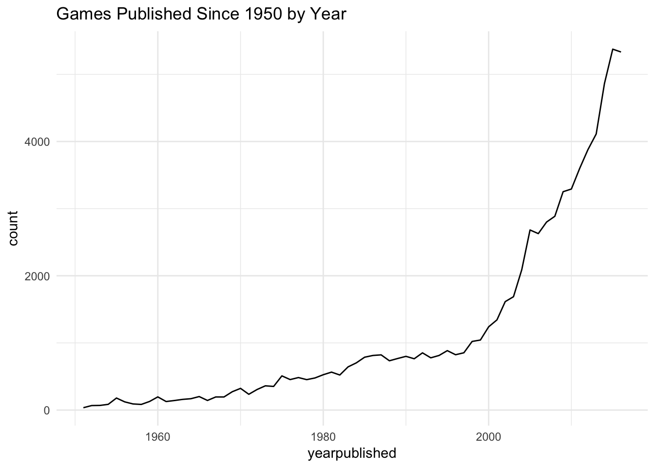

Publishers Over Time

We can see a similar increase in the number of publishers.

publishersOverTime <- gamesDf %>%
  group_by(yearpublished) %>%
  summarise(
    publisherCount = n_distinct(boardgamepublisher)
  )
ggplot(data = publishersOverTime, aes(x = yearpublished, y = publisherCount)) +
  geom_line() + theme_minimal()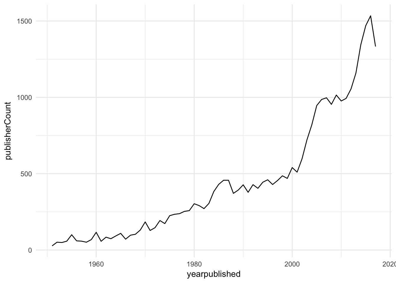

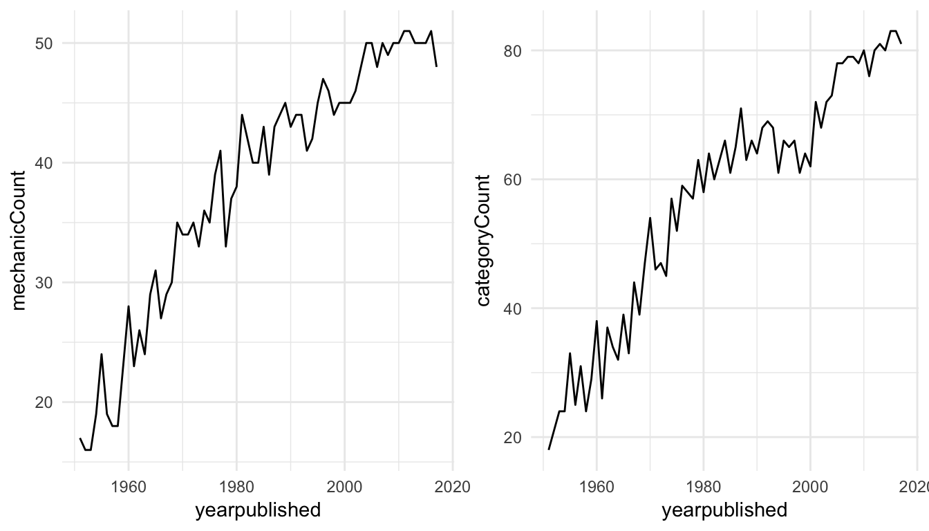
Mechanics and Categories Over Time

Not only are we getting more games from more publishers, but the games that are being published are richer in terms of mechanics (tags describing how the game is played, like ‘dice rolling’, or ‘tile placement’), and categories (tags describing what the game is about, like ‘Civil War’, or ‘Racing’).

mechanicsOverTime <- gamesDf %>%
  group_by(yearpublished) %>%
  summarise(
    mechanicCount = n_distinct(boardgamemechanic)
  )
mechanicsPlot <- ggplot(data = mechanicsOverTime, 
                        aes(x = yearpublished, y = mechanicCount)) +
  geom_line() + theme_minimal()

categoriesOverTime <- gamesDf %>%
  group_by(yearpublished) %>%
  summarise(
    categoryCount = n_distinct(boardgamecategory)
  )
categoriesPlot <- ggplot(data = categoriesOverTime, 
                         aes(x = yearpublished, y = categoryCount)) +
  geom_line() + theme_minimal()

gridExtra::grid.arrange(mechanicsPlot, categoriesPlot, ncol = 2)

Mechanics Over Time

November 9, 2017

board games R statistics

Getting boardgamegeek Data

October 30, 2017

R web scraping boardgames

Publishing Trends

November 17, 2017